Playing with large set of data is always fun if you know how to do it. You can fetch interesting information from it. As part of my Master’s course I have had opportunity to work on forecasting using Times Series modeling. And yes, now I can predict future without being a clairvoyant. 😀

Considering popularity of R in Data Science, I started with R. But soon I realized it has learning curve. So, I opt out for Python. I am not going to write R vs Python because it is already written nicely here in DataCamp’s blog.

So, let’s get started. Time series models are very useful models when data points collected at constant time intervals. This time series stationarity is main per-requisite for the dataset. Until unless your time series is stationary, you cannot build a time series model. There is a popular example named “Random Walk”. The summary of the example is prediction becomes more inaccurate as input data is randomize.

We will use two completely different dataset to for prediction.

• Nile Water Level between AD 622 to AD 1284. Get it here
• Air Quality data of Italy taken on Hourly basis. Get it here

The reason we are taking two different model because we want to show multiple different Time Series models.

ARMA:

ARMA is basically combination of two different time series model AR and MA. AR stands for Auto Regressive and MA stands for Moving Average. In ARMA we work with single dependent variable indexed by time. This method is extremely helpful when we do not have any other data than time and one specific type of data. For example in case of Nile data we only have the water level data which is indexed by time(year). I am giving you warning, if your data is not stationary you will be tearing off all of your hair to fit the model. So, make sure your data is consistent to save your hair.

We have used Pandas for Data management.

We have used StatsModels ARMA method for prediction. It takes an mandatory parameter order which defines two parameters p,q of ARMA model. p is the order for AR model and MA is for MA model. Full API reference for this function can be found here. StatsModels also provides ARIMA modeling. In case of ARIMA model we just have to pass difference order parameter.

The predictors depend on the parameters (p,d,q) of the model. Here is the short description about it.

1. Number of AR (Auto-Regressive) terms (p): AR terms are just lags of a dependent variable. For example if p is 5, the predictors for x(t) will be x(t-1)….x(t-5).
2. Number of MA (Moving Average) terms (q): MA terms are lagged forecast errors in prediction equation. For example if q is 5, the predictors for x(t) will be e(t-1)….e(t-5) where e(i) is the difference between the moving average at the i^th instant and actual value.
3. Number of Differences (d): These are the number of nonseasonal differences, i.e. in this case we took the first order difference. So either we can pass that variable and put d=0 or pass the original variable and put d=1. Both will generate same results.

To calculate p and q I have run Autocorrelation Function (ACF) and Partial Autocorrelation Function (PACF). StatsModels have acf and pacf function to do this for us.

How I have done it:

At first, I have installed Anaconda to get everything I need. Yes. we have gathered the whole zoo to do our data science. Python, Pandas and now Anaconda. Don’t forget you can write your code in IDE named Spider. Whatever…

After that, I have used Pandas to read CSV. At first I was trying to fit ARMA on Air data. But since it was hourly data, fitting those data was difficult. Then I moved to Nile data. I was having hard time fitting Nile data because the time span for the data was out of the range of supported timestamp. So, instead of using DateTime index I switched to period range of Pandas. I have generated custom period range to support the time range. The while fitting ARMA model I passed the dates generated by the period range with annual frequency. For p and q order I have used ACF and PACF. I have calculated the lags and then plot it on a graph with bounds.

ACA and PACA observation

Observing the graph I have taken (2,2) as (p,q) order. After fitting the model I have predicted using the model. Here is the output of the prediction:

Nile Water level prediction

Linear Regression & Random Forrest Regression:

Besides ARMA and ARIMA model we have tried to use other prediction model. One of them are Linear Regression. SciKitLearn provides handful methods to do Linear Regression and Random Forrest Regression. I have ran these models on Air Quality data and got very good output. It has been observed that Random Forrest Regression generates more accurate predictions than Linear Regression. Random Forrest Regression has error rate of 12.8169340263% where as Linear Regression generates output with error rate 29.8718180357%.

How I have done it:

After reading data from CSV using pandas I have dropped NA(not available) or null values. Then I have omitted extreme values. I have run a co-relation calculation with all the columns against Temperature. The output was following:

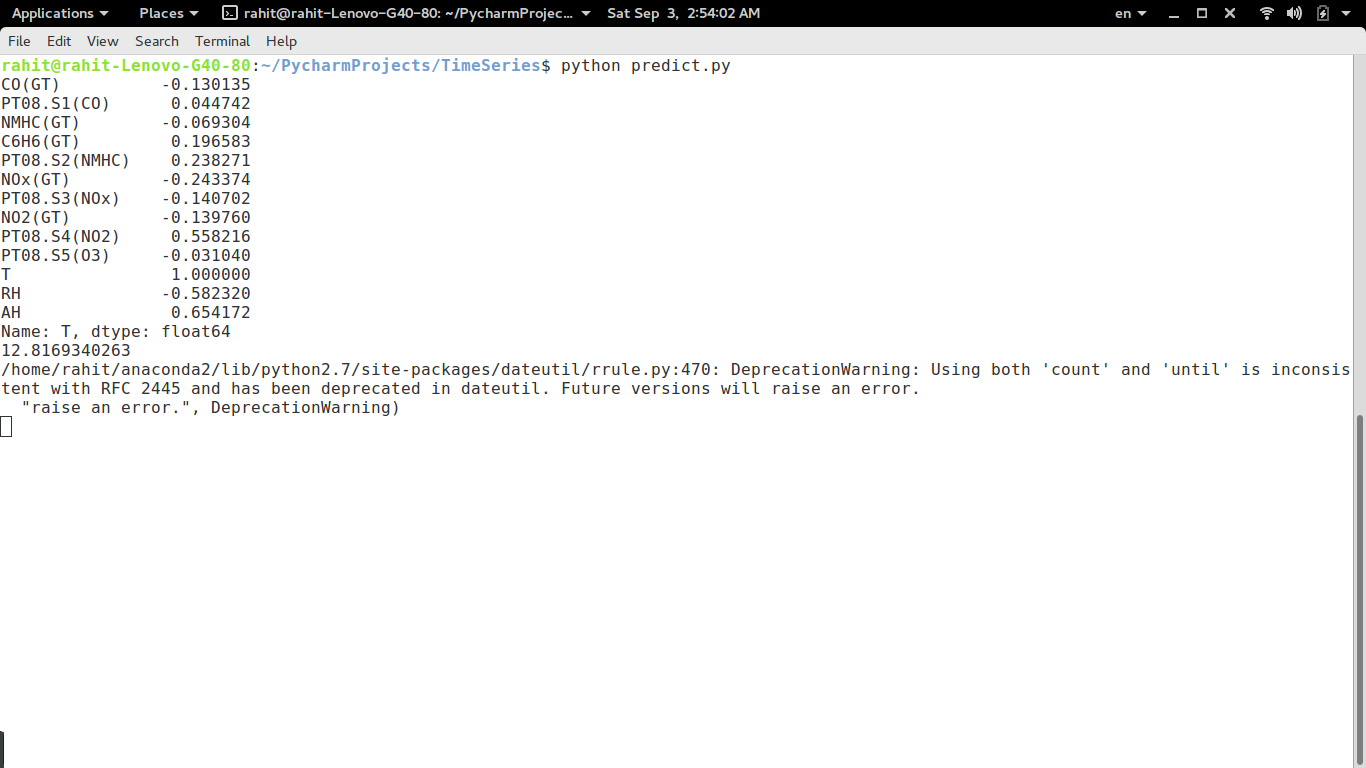
Correlation with Temperature

Then I have run prediction model on on the data. I have considered Temperature “T” as the dependent variable and others as the independent variable. The output was following:

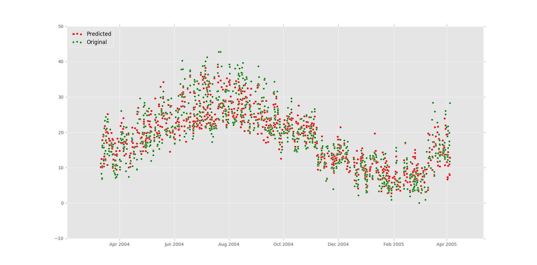
Random forest

Here is the code for everything I described above.